Introduction
While reading about game AI or game development, I often come across statements like these:
- “A common algorithm to find the path is A* (pronounced “A star”), which is what Unity uses.”[1]
- “The A* pathfinding algorithm is often a starting point for pathfinding approaches in games but can be then built into more hierarchical or optimized frameworks, such as D* or D* Lite to serve specific game design challenges.” [2]
- “A* is often used for the common pathfinding problem in applications such as video games, but was originally designed as a general graph traversal algorithm.” [3]
I’ve reread it so many times that I was under the impression that I understood how pathfinding works. It’s magic! A crystal ball called A* can generate a path when you ask for it. Well, sometimes, that’s just enough. But more often than not, we need to change how an NPC moves, and for that, an understanding of how the algorithm works can be useful. So let’s try to understand A* together and see what can be done with that.
Table of contents
Open Table of contents
Graphs, costs, and definitions
3D geometry might not be the easiest example for understanding how a pathfinding algorithm works, so I’m going to use something simpler. This is a node graph, where each node represents a place (like a city), and the lines between represent connections — like roads between those cities. For this post, I’m going to use a graph made up of 8 nodes, each named with a letter.
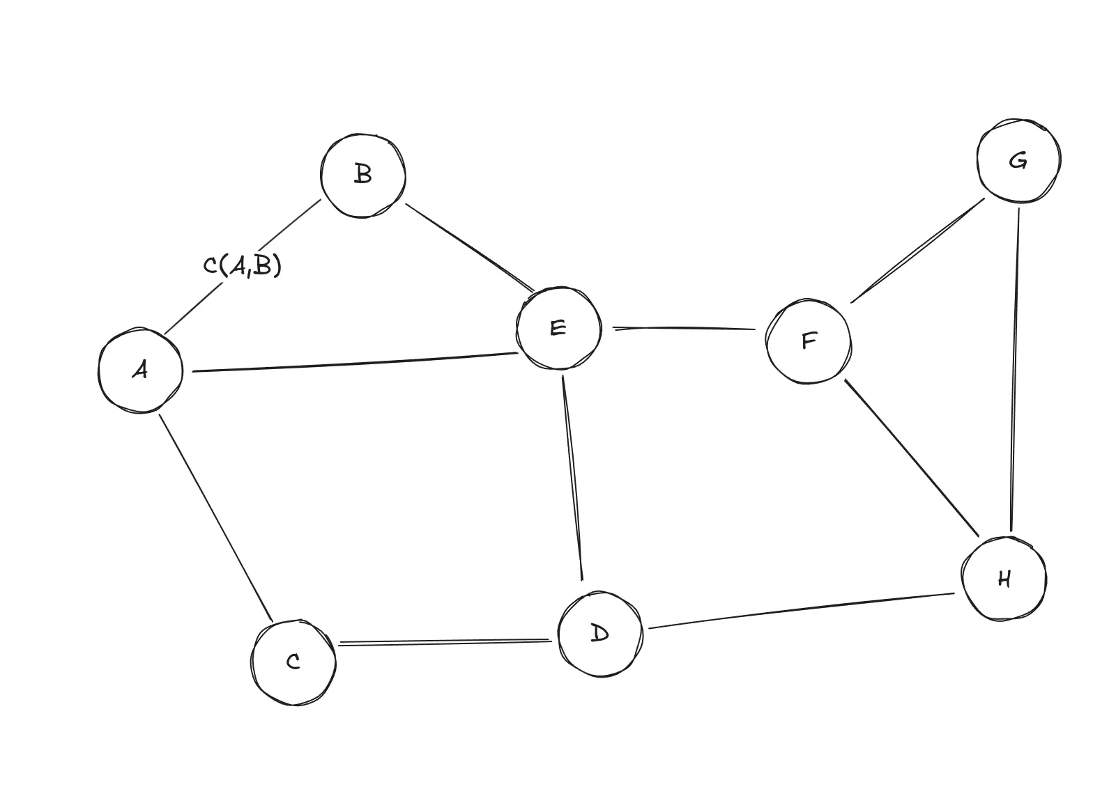 Search space representation in the form of a graph. The cost of traversing between the nodes A and B is .
When traversing a graph, we have to pay a cost. In real life, we do the same, except the cost is usually distance or time. In general, the cost of traversing from one node to another can be expressed as . Read it as a cost of traversing from a node to a node . You can see it marked between the nodes and .
When traversing multiple nodes, we create a path. A path also has a cost, calculated as the sum of the costs between the individual nodes in the path.
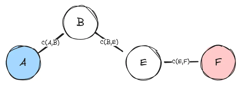 Figure showing a simple path from node to node . The cost of the path shown in the figure is .
Basic pathfinding
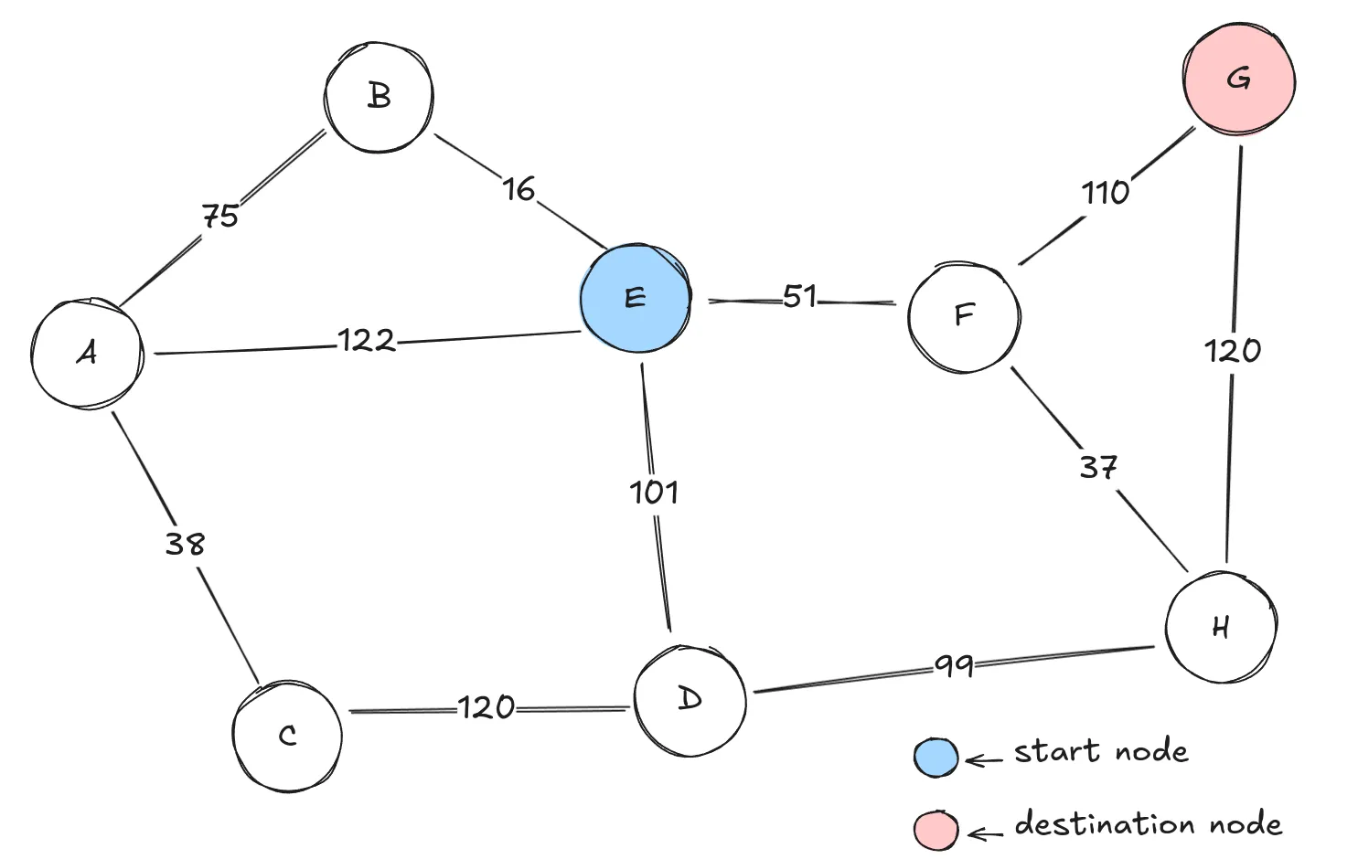 Graph with costs between the nodes, a start node, and a destination node marked.
In this example, the goal is to find the shortest path between the nodes and , assuming that we don’t know anything about the world in which we are searching. Just imagine that you are in a foreign country without a map, and you find out that city B is connected to cities A and E once you get there.
At node , there are four options to choose from: . But which do we select? We could always choose the node that results with the shortest path. If we kept doing this, we’d eventually reach node , and we could be certain that the path we found had the smallest possible cost — in other words, the path would be optimal.
Let’s try this out! At every step of the iteration I’m going to choose a path that yeilds the smallest cost
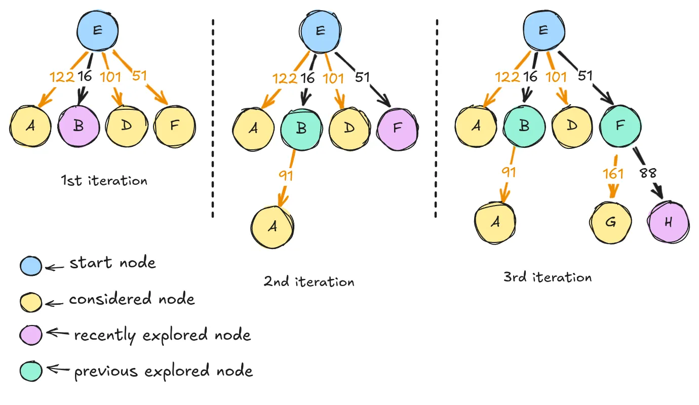 First three steps of the iteration performing Dijkstra’s algorithm.
Pretty simple, right? At the first step, we chose node , because the path from it to the node costs 16. At the next step, we see one “new” node, . We start again, we evaluate every path from the start. But the shortest path is not , it’s , so we explore the node . In the third step, we repeat the same operation, we evaluate path to every node that hasn’t been explored, and we choose the shortest. All pretty straightforward.
This simple approach has its formal definition in mathematics. Imagine an evaluation function that takes a node as an input and returns a number. Each time we have to select a node, we’ll choose the one with the smallest value of that function. In our case, the evaluation function is going to return the cost of traversing from the start node to node . This exact approach in AI literature is called uniform-cost search, but you might also have heard about it under the name Dijkstra's algorithm. [4]
In general, any algorithm that uses an evaluation function to guide its search is called best-first search, since we select the node that best fits our approach.
The problem with uniform-cost search is that it explores a lot of nodes. As it prefers low-cost moves, it will explore many of them before considering higher-cost ones. Another issue is that it evaluates — and even explores — nodes that aren’t leading toward the destination. For a small graph, it doesn’t matter. But if we had a large scene and only a fraction of the CPU time dedicated to pathfinding, this could become a bottleneck.
A*
In many cases, and especially in video games, we have information about the world that can help guide pathfinding. An algorithm could make assumptions about the search space, and use them. Methods that apply this are called informed search algorithms. What kind of assumptions we make as its authors, and how we use them, is up to us.
A* is an informed, best-first search algorithm that uses an evaluation function:
Where:
- is the evaluation function of a path that goes from to a goal.
- is the path cost from the initial state to node ,
- is the assumption about the world, it’s called the heuristic function.
A*uses the shortest path from to a goal node.
It might sound confusing. How can we get the estimated cost of the shortest path from n to the goal state? In reality, the cost of the shortest possible path between two points is the distance between those points. So A* selects nodes based on the cost of the path and the distance to the destination.
In games, we can calculate that distance quite easily. With this in mind, let’s revisit our example.
Again, we will consider the path from node to the path . Here’s a table of distances from our goal point to any of the nodes:
| Node | Distance (from G) |
|---|---|
| A | 162 |
| B | 140 |
| C | 122 |
| D | 87 |
| E | 66 |
| F | 36 |
| G | 0 |
| H | 60 |
A table containing all the distances from any node to node G
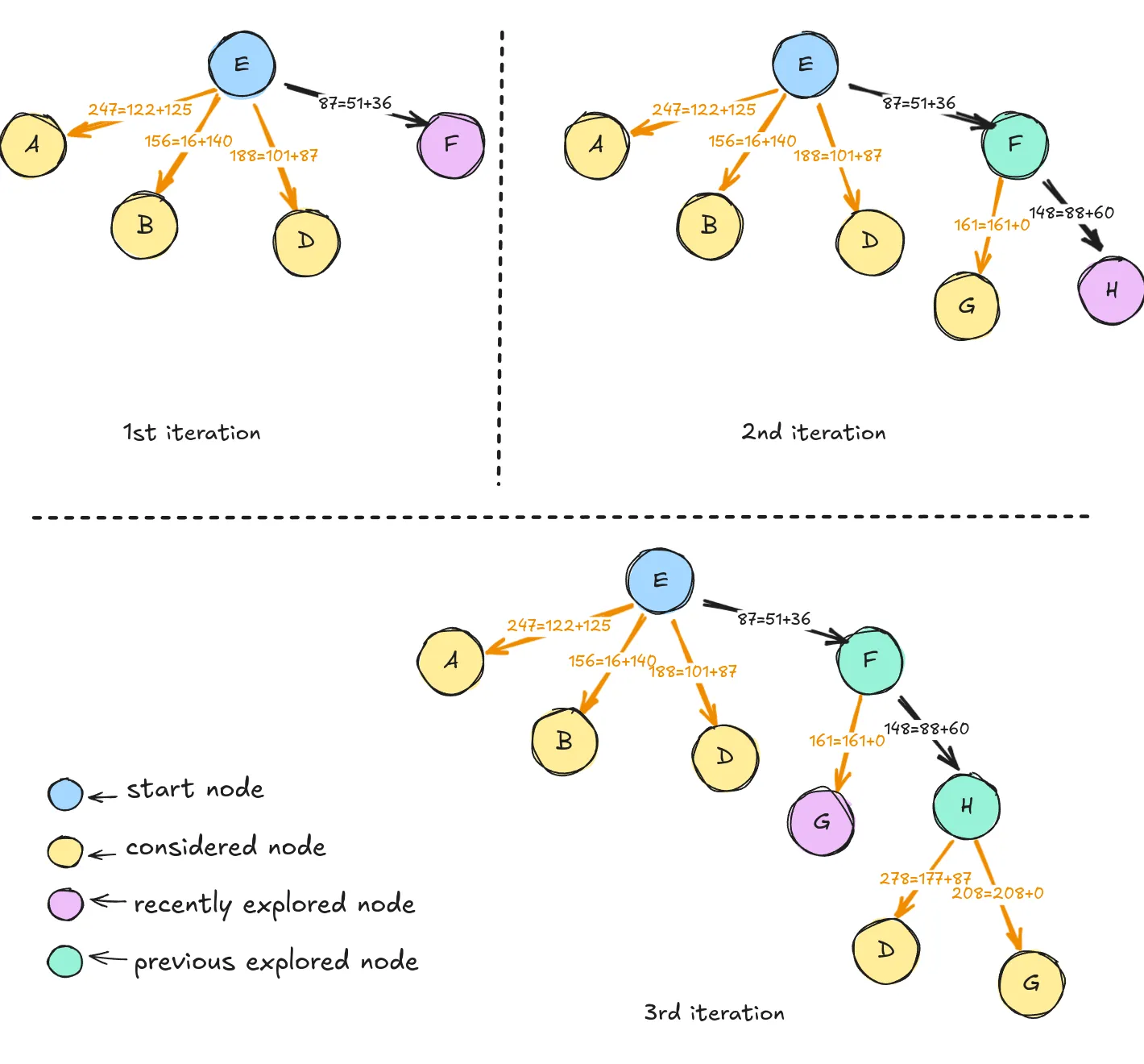 The first three stages of
 A* search for a path from to . Arrows are labeled with the evaluation function
Notice the improvement of the algorithm, the optimal path was found in just three steps. Generally speaking, A* is performant because it removes of the possibilities without examining them. This is called pruning, and it is a common technique in artificial intelligence. [4]
Just like uniform-cost search, A* guarantees to find an optimal path if it exists, which means that it is complete and cost-optimal, but it is not perfect.
(Un)real-life examples
Let’s shift the analysis from graphs to something that looks like a video game.
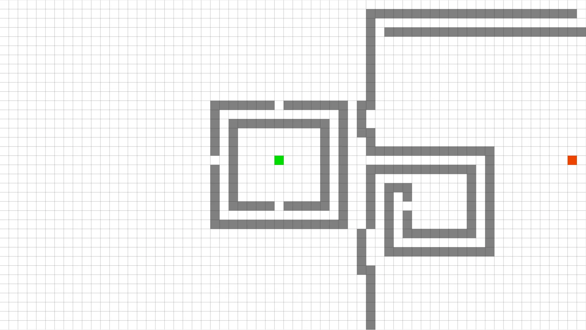
This is a screenshot from a tool [5] that visualizes pathfinding algorithms. Have a look on how Dijkstra’s algorithm behaves:
It explores the environment very uniformly, expanding like circular waves around a source. It took 11.5 seconds and 4117 operations to find the optimal path (115.84). We already know that it is slow, so let’s see how it compares to A*.
It’s better, notice how it is pulled towards the goal. It found the same path in 8.7 seconds, making 3295 operations. We can say that in this case, we have a 20% improvement. But still, A* explored a lot of nodes and took quite a lot of time. Depending on the problem and the device we’re working with, that might be good enough — but what if it’s not?
The imperfect solution
We can improve A*’s performance if we are willing to sacrifice the perfection of the path, we just have to tweak the algorithm a little bit. If you have a look at the video with A* solving the map, you might notice that it considered a lot of nodes that weren’t in the direction of the solution. What if we could change how it treats the nodes closer to the solution, and make them more important — or, mathematically speaking, increase the weight of the heuristic function, we could do it like so:
This approach is called Weighted A*, and it generalizes the best-first search.
With , we can control how much the heuristic influences the search. Have a look at the same map with .
Weighted A*, with found a suboptimal solution (117.36) in 3.3 seconds and only 2244 operations. This is a 45% improvement if we compare it to Dijkstra’s algorithm, which is a great result!
I think that this is a great tread-off. Space and time performance are things we often have to fight for — and sacrificing a bit of quality (which the end user won’t even notice) can be a smart decision. Also in some cases, we don’t even want optimal solutions. In pathfinding, a little randomness can be a good thing — it can make agents look more human. I think this is obvious for anyone who makes AI agents or even plays video games: humans aren’t perfect, so NPCs shouldn’t either.
Not only we can use the heuristic to speed up pathfinding, but we can also manipulate it in ways that benefit our game. If we treat the weight as a function instead of a constant, we could change it dynamically — increasing the cost of traversing certain areas, even banning NPC from entering them. For example, stopping an evil creature from walking onto holy grounds.
Conclusion
I hope that these explanations show you that Dijkstra's algorithm, A* and Weighted A* are closely connected and you can experiment with them. For me understanding how they work makes them feel like tools that I can play with. That’s something I want to have more — knowledge of how to use mathematics and technology to create something interesting!
Bibliography
- https://docs.unity3d.com/510/Documentation/Manual/nav-InnerWorkings.html
- Roberts, P. (Ed.). (2024). Game AI Uncovered: Volume One (1st ed.). CRC Press. https://doi.org/10.1201/9781003324102
- https://en.wikipedia.org/wiki/A*_search_algorithm
- Russell, S. & Norvig, P. (2021). Artificial Intelligence, Global Edition. (4th ed.). Pearson Education. https://elibrary.pearson.de/book/99.150005/9781292401171
- https://qiao.github.io/PathFinding.js/visual/.