How A* Sees the World; An Introduction to Navigation Meshes

Preface

The idea for this article came to my mind after finishing the last entry, where I asked myself, “How exactly does A* get information about a scene?” This simple but important question bothered me so much that I decided to explore it.

Although I’ve used or interacted with a NavMesh thousands of times, I had never asked myself how it works. I think that in complex systems, we stop paying attention to parts that just work.

Navigation Mesh is a mature concept that solves problems most people had forgotten even existed. It was exciting for me to step into the shoes of people who had to solve these problems in the first place.

Prerequisites

You should be familiar with A*. I recommend reading my previous post where I explain A* within a wide context.

Introduction

Let’s step back a little and take a different perspective: imagine there’s no NavMesh implementation. How would we make pathfinding work? This question requires us to solve three main problems. First, we need to pass the information to the pathfinding algorithm. Secondly, we must do it efficiently so we don’t destroy our game’s performance. Finally, we have to consider the validity of the path. Let’s go through them one by one.

Table of contents

Feeding the algorithm

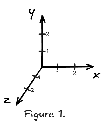
At the center of any scene is a Cartesian coordinate system. We use it to express positions, measure distances, and have a center we can relate to.

A coordinate system uses real numbers. If you remember from your math lessons, the set of real numbers has infinitely many elements. On one hand, this is great because it gives us infinite precision for expressing positions. On the other hand, it’s a problem because a pathfinding graph cannot have an infinite number of nodes. Even if we were to limit the coordinate space to the furthest position in a scene in each dimension, we still would be working with an infinitely sized set.

You might say that this is not technically correct, since computers are physical machines with finite precision, and they cannot express all real numbers. You’d be right. However, with 32 bits (typical size of float) we have $2^{32} \approx 4\space294\space967\space296$ distinct bit values just in one dimension. We might as well treat it as a set with an “approximately” infinite number of elements.

This points out an old but fundamental problem: how do we express a continuous or an extremely large set with a finite set? Fortunately, people who deal with signal processing have figured it out a long time ago; the answer is quantization.

Quantization

Quantization expresses continuous values using a finite set of approximated values. Although approximation helps us immensely with expressing these values, it introduces errors. Figure 2 shows an example of quantizing a sine wave.

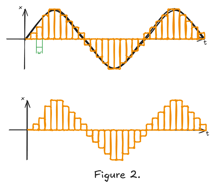
I won’t detail the math of this process, but you can see that the rectangles have a constant width and a height which represents the signal value. We can fit a fixed amount of these fixed-width rectangles, meaning they don’t follow the curve perfectly. This is important, and we are going to come back to this later.

The same approach can be applied to a scene. We can subdivide it into square shaped cells of length $\Delta l$, essentially repeating the same process as with the sine wave but in two dimensions.

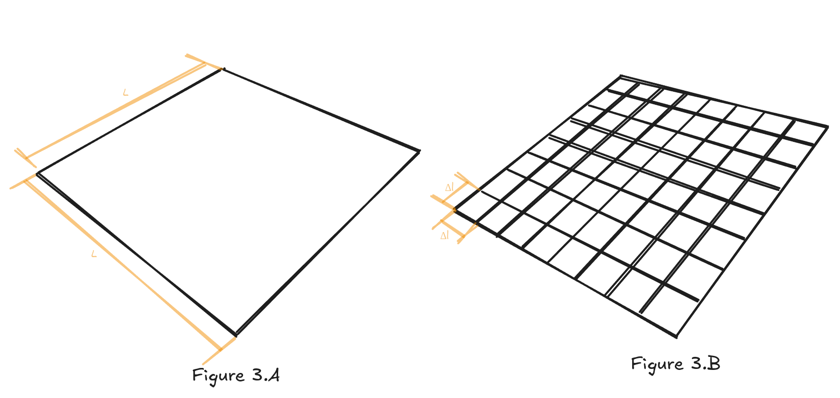
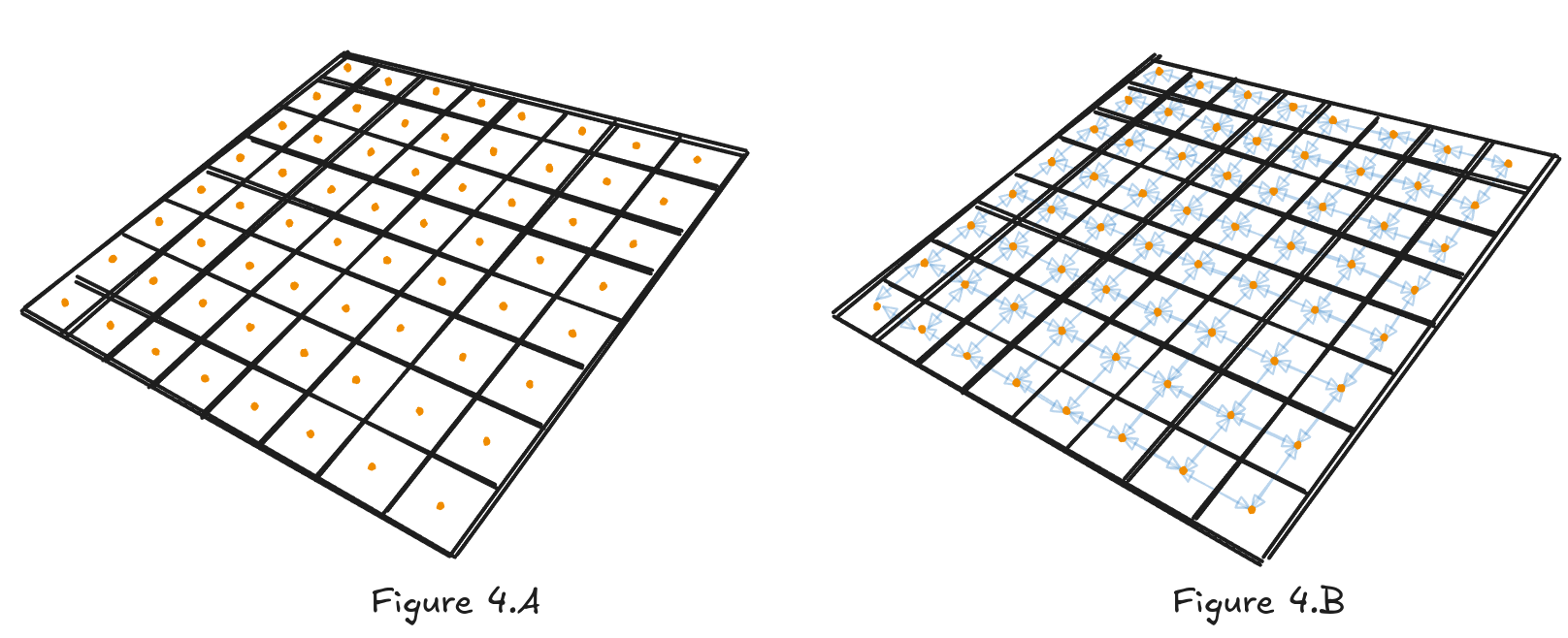
In this subdivided form, by placing a node in the middle of each cell, we are essentially getting a square graph, which we can feed into a pathfinding algorithm. This approach is called Grid Graph; it’s a simple way of doing pathfinding.

Since each node connects to its closest neighbors, they can have two, three, or four edges. The cost of traveling between any adjacent nodes can be calculated as a function of distance between their positions or the traveling time between them.

Searching the path

What happens if we want to do a search from point $A$ to $B$ where none of the points are in the center of the cell? We are going to approximate their positions to the closest nodes (see Figure 5.A). As I said before, quantization introduces errors. We can influence the error by decreasing the size of $\Delta l$, but this increases the number of nodes.

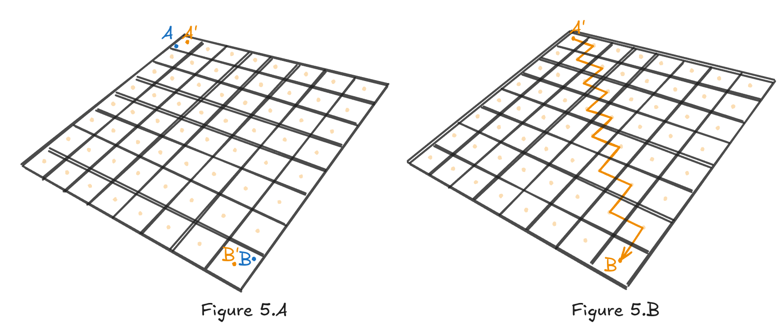
With positions corresponding to nodes, we finally have a form that matches A*’s or any other pathfinding algorithm’s expectations. We perform the search and get back path $p$ (see Figure 5.B).

The path is unfortunately very angular; it changes heading at every node. An agent taking this path would look very unnatural. This situation could be fixed if we allowed for 8-directional connections instead of four. It would make a straighter path, but it would nearly double the number of edges (by 77% according to my calculations). Another option is to smooth out the path, which we will cover later. Now, let’s look at a different case.

Validity

The previous example is incredibly optimistic in terms of elements in a scene. In order to truly evaluate this technique, we have to see how it would behave, at least, in an average scenario: a scene with one building. Figure 6.A shows a plane with a rectangular building on it and three distinct points $n_1$, $n_2$, and $n_3$.

Although point $n_3$​ is on walkable ground, its cell’s center is blocked, making the node invalid. We cannot perform a search to it because that would result in an invalid path.

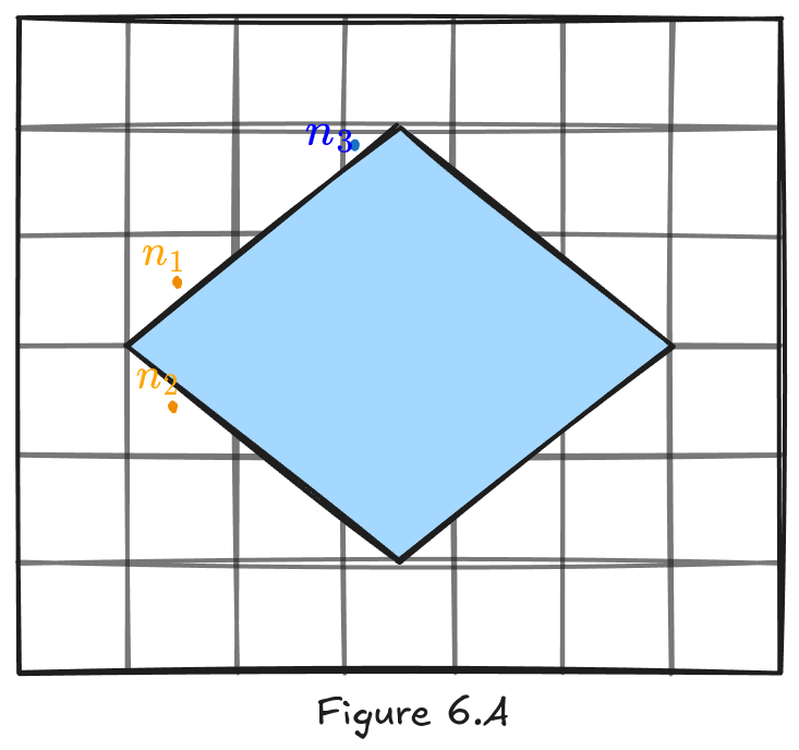
There’s another difficult case here: points $n_1$ and $n_2$. Let’s say we want to move from one to another. Since they are both in the center of the node, the algorithm can solve a path between them. The shortest path between those two points is a straight line. An NPC following this path would collide with the wall, this is not good. The issue can be mitigated if we increase the resolution of the graph and use smaller cells. While fixing this, I increased the number of cells twenty five times for Figure 6.B.

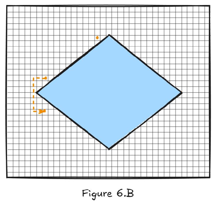
Grid graphs are simple and straightforward implement; however they require high resolution to accurately represent objects that don’t lie on a grid.

Navigation meshes - what is it exactly?

Division schemes are ways of abstracting a scene into a format that’s useful for processing, it can be pathfinding or other spatial reasoning. So far we’ve talked about grid graphs, but they are other ways of doing this: Dirichlet Domains, Points of Visibility, or finally, Navigation Meshes. They are the de facto standard of the industry.[3]

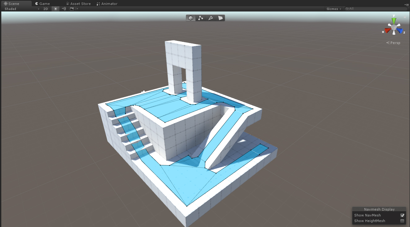
Navigation mesh , or NavMesh, is a search space optimization built from a scene. Like a grid graph, NavMesh is used as an abstraction of a scene; it can be used for feeding the pathfinding algorithm. It takes the form of a static mesh, built in the editor after the level geometry has been laid out. Just this fact is a major improvement over Grid Graphs. Since there’s no information about the areas that weren’t marked as walkable, the game doesn’t have to check if a cell is blocked by a static geometry or not, which makes it mostly valid. In other words, if you can’t walk on it, it has no NavMesh.

The process of generating a Navigation Mesh is called baking. Either the rendering or the physics geometry can be used for baking, but the latter option is chosen more often. Why? Nowadays physics geometry, aka. colliders, is much simpler in comparison to rendering geometry. Additionally, they are the source of truth for the physics engine which controls most of the object in a scene. Despite what’s used, the resulting mesh is constructed from polygons, usually triangles, but quads are also a valid option.

How a NavMesh is baked and what influences its generation are interesting topics themselves. Things like agent size, the NavMesh’s maximum and minimum allowed slope, or even the minimum size of a created region are all configurable in most engines. However, I’ll focus only on the basic ideas behind NavMesh for now, so I’ll ignore those low-level details.

Characteristics

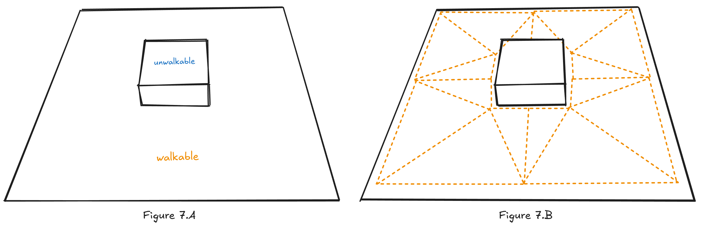
Figure 7.A shows a simple scene with a walkable floor and a box that’s unavailable for the navigation system. The drawing to the left shows how a Navigation Mesh would look after being baked (the process of generating the NavMesh is called baking) from the scene. You can see immediately see there are fewer triangles than there were squares in a grid graph.

A pathfinding graph is created by placing a node in the center of each polygon. Any two nodes are connected if the corresponding polygons share an edge. Notice the difference between NavMesh and the grid graph.

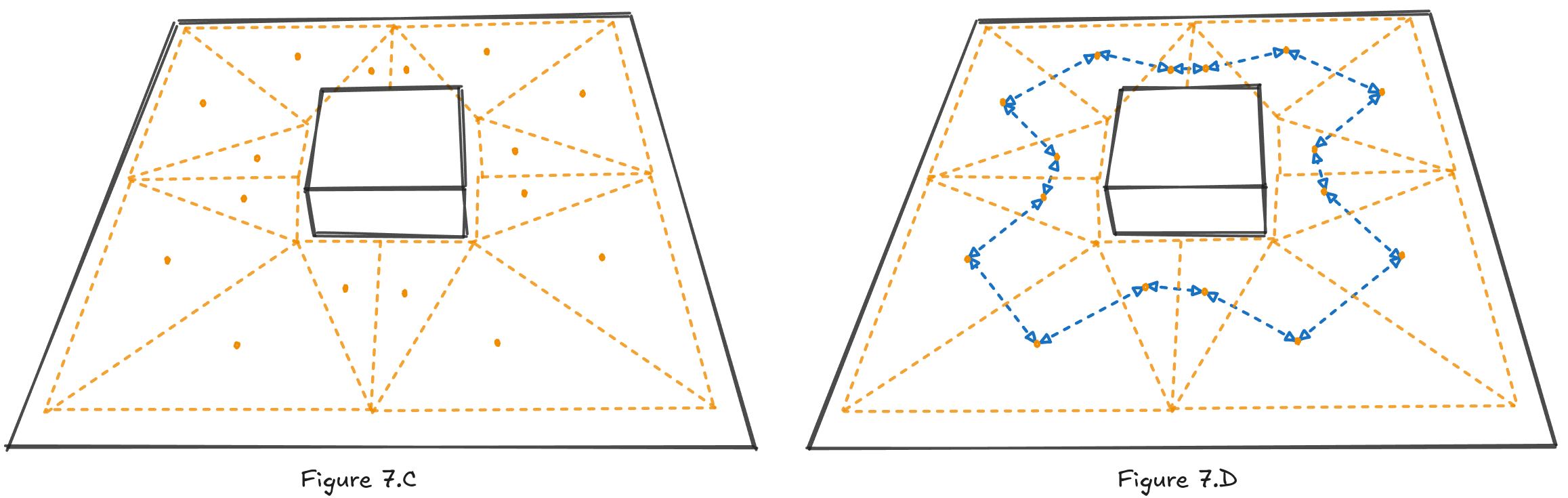
Just like with Grid Graphs, when searching, positions are first quantized to a node in the graph. This process of matching positions and nodes is simple in theory for Navigation Meshes. We just have to check which triangle contains the requested position, whether it’s the start or finish position.

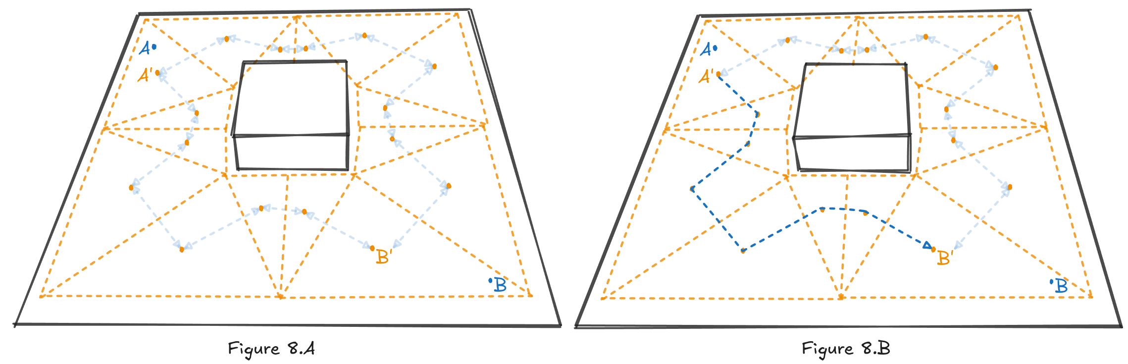
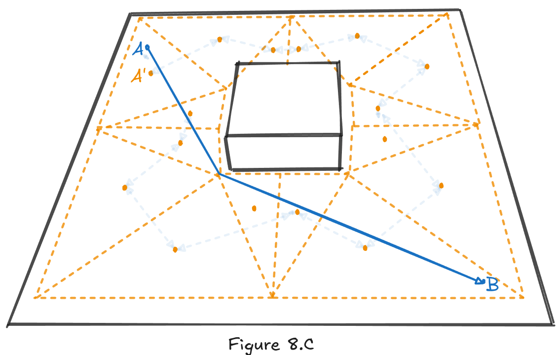
A*, or any other pathfinding algorithm, operates in something that I would call the graph space. It has no information about the game world; it only has information about the graph. The graph itself is made out of nodes, edges and cost functions, but they are only an abstraction of the real world. For us this means three things:

• First, the search is bound to the nodes (see Figure 8.B).
• Second, any optimization introduces errors.
• Third, the path has to be converted back to the game space.

String-pulling based smoothing

Introduction

The last two things we have to do are smooth out the path, and make it relative to the game world. As always there are multiple ways of doing things, String-Pulling Approach is the industry standard. [https://idm-lab.org/bib/abstracts/papers/socs20c.pdf]

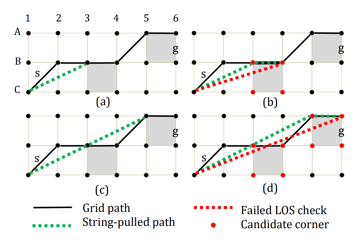
Introduced by Han et al. [2], String Pulling is an algorithm for smoothing out paths. You can imagine it working as if we were to pull a piece of string between the start and end points. The shape that the string would have would be the shortest path between two points.

The authors of the paper added a benchmark for the algorithm against different versions of A* and a more sophisticated pathfinding algorithm, Theta*. The string-pulling approach introduced a minor runtime overhead, increasing the average time by 2%. The path length deviated by around 0.47% from the calculated reference. In comparison, raw A* extended the path by 4.73%. Last, but not least, string-pulling on average removed all unnecessary heading changes, it even beat Theta*.

![[Pasted image 20250701153840.png|1000]] **

How does it fit together?

The sequence of nodes that’s returned from A* is transformed to a sequence of positions. Start and finish positions are added to that sequence with an assumption that there is a direct line of sight, from the node centre to that position. Then the path is smoothed out, which means, that it’s shorter, has fewer unnecessary turns and just looks better.

Summary

In this post, we talked about how A* gets information about a scene, and what the basic concepts behind quantization are. We followed the simplest approach (Grid Graphs) for abstracting the scene and found issues with that. We moved from Grid Graphs to current techniques called Navigation Meshes, and, we discussed the entire pathfinding process with these meshes.

Conclusions

For me, grasping the core problem allows me to understand the tool or method that I’m using. And I hope with this entry I have achieved the same for you. This blog post is by no means a complete description of what can be achieved with NavMeshes. There are other topics like: generation, multiple agents, dynamic obstacles, moving NavMeshes, etc. I encourage you to try reading and playing with those concepts on your own.

Bibliography

1. https://en.wikipedia.org/wiki/Quantization_(signal_processing)
2. https://idm-lab.org/bib/abstracts/papers/socs20c.pdf
3. Millington, I. (2019). AI for Games, Third Edition (3rd ed.). CRC Press. https://doi.org/10.1201/9781351053303
4. https://www.wikiwand.com/en/articles/Navigation_mesh
5. https://www.wikiwand.com/en/articles/A%2A_search_algorithm
6. https://dev.epicgames.com/documentation/en-us/unreal-engine/basic-navigation-in-unreal-engine